Qubit spectroscopy: \(T_1\) measurement example

This notebook demonstrates how to use the module qubit_spectroscopy to assess the “energy relaxation” time, \(T_1\), of one or more qubits on a real quantum device using pyQuil. This one of the major sources of error on a quantum computer.

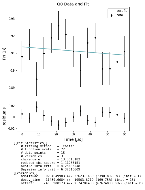
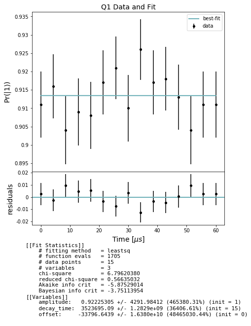
A \(T_1\) experiment consists of an X pulse, bringing the qubit from \(|0\rangle\) to \(|1\rangle\) (the excited state of the artificial atom), followed by a delay of variable duration.

The physics of the devices is such that we expect the state to decay exponentially with increasing time because of “energy relaxation”. We characterize this decay by the decay_time constant, typically denoted \(T_1 =1/\Gamma\) where \(\Gamma\) is the decay rate. The parameter \(T_1\) is referred to as the qubit’s “relaxation” or “decoherence” time. A sample QUIL program at one data point (specified by the duration of the DELAY pragma) for qubit 0 with a 10us wait would look like

DECLARE ro BIT[1]
RX(pi) 0
PRAGMA DELAY 0 "1e-05"
MEASURE 0 ro[0]

NB: Since decoherence and dephasing noise are only simulated on gates, and we make use of DELAY pragmas to simulate relaxation time, we cannot simulate decoherence on the QPU with this experiment as written. This notebook should only be run on a real quantum device.

setup - imports and relevant units

from matplotlib import pyplot as plt
from pyquil.api import get_qc, QuantumComputer

from forest.benchmarking.qubit_spectroscopy import (
    generate_t1_experiments,
    acquire_qubit_spectroscopy_data,
    fit_t1_results, get_stats_by_qubit)

We treat SI base units, such as the second, as dimensionless, unit quantities, so we define relative units, such as the microsecond, using scientific notation.

MICROSECOND = 1e-6

Get a quantum computer

# use this command to get the real QPU
#qc = get_qc('Aspen-1-15Q-A')

qc = get_qc('2q-noisy-qvm') # will run on a QVM, but not meaningfully
qubits = qc.qubits()
qubits

[0, 1]

Generate simultaneous \(T_1\) experiments

We make and experiment for each desired qubit in qubits, specifying the times in seconds at which we would like to measure the decay.

import numpy as np
stop_time = 60 * MICROSECOND
num_points = 15
times = np.linspace(0, stop_time, num_points)
expt = generate_t1_experiments(qubits, times)
print(expt)

[<forest.benchmarking.observable_estimation.ObservablesExperiment object at 0x7fc7f79202e8>, <forest.benchmarking.observable_estimation.ObservablesExperiment object at 0x7fc7f7920588>, <forest.benchmarking.observable_estimation.ObservablesExperiment object at 0x7fc7f7920898>, <forest.benchmarking.observable_estimation.ObservablesExperiment object at 0x7fc7f7920ba8>, <forest.benchmarking.observable_estimation.ObservablesExperiment object at 0x7fc7f7920e80>, <forest.benchmarking.observable_estimation.ObservablesExperiment object at 0x7fc7f78c4198>, <forest.benchmarking.observable_estimation.ObservablesExperiment object at 0x7fc7f78c4438>, <forest.benchmarking.observable_estimation.ObservablesExperiment object at 0x7fc7f78c4748>, <forest.benchmarking.observable_estimation.ObservablesExperiment object at 0x7fc7f78c4ac8>, <forest.benchmarking.observable_estimation.ObservablesExperiment object at 0x7fc7f78c4dd8>, <forest.benchmarking.observable_estimation.ObservablesExperiment object at 0x7fc7f78c9128>, <forest.benchmarking.observable_estimation.ObservablesExperiment object at 0x7fc7f78c9438>, <forest.benchmarking.observable_estimation.ObservablesExperiment object at 0x7fc7f78c9748>, <forest.benchmarking.observable_estimation.ObservablesExperiment object at 0x7fc7f78c9a58>, <forest.benchmarking.observable_estimation.ObservablesExperiment object at 0x7fc7f78c9d68>]

Acquire data

Collect our \(T_1\) raw data using acquire_qubit_spectroscopy_data.

num_shots = 1000
results = acquire_qubit_spectroscopy_data(qc, expt, num_shots)

Analyze and plot

Use the results to produce estimates of :math:`T_1`

In the cell below we first extract lists of expectations and std_errs from the results and store them separately by qubit. For each qubit we then fit to an exponential decay curve and evaluate the decay_time constant, i.e. the T1. Finally we plot the decay curve fit over the data for each qubit.

from forest.benchmarking.plotting import plot_figure_for_fit

stats_by_qubit = get_stats_by_qubit(results)
for q, stats in stats_by_qubit.items():
    fit = fit_t1_results(np.asarray(times) / MICROSECOND, stats['expectation'],
                         stats['std_err'])
    fig, axs = plot_figure_for_fit(fit, title=f'Q{q} Data and Fit', xlabel=r"Time [$\mu s$]",
                           ylabel=r"Pr($|1\rangle$)")
    t1 = fit.params['decay_time'].value # in us