Quantum Volume
The quantum volume is a holistic quantum computer performance measure [QVOL0, QVOL1, QVOL2].
Roughly the logarithm (base 2) of quantum volume \(V_Q\), quantifies the largest random circuit of equal width and depth that the computer successfully implements and is certifiably quantum.
So if you have 64 qubits and the best log-QV you have measured is \(\log_2V_Q = 3\) then effectively you only have a 3 qubit device!
The quantum volume metric accounts for all relevant hardware parameters, e.g.
- coherence
- calibration errors
- crosstalk
- spectator errors
- gate fidelity, measurement fidelity, initialization fidelity
- qubit connectivity
- gate set
Some details
A circuit that measures the quantum volume consists of layers of a permutations of \(n\) qubits followed by nearest neighbor two qubit Haar random unitaries. At the end we measure in the computational basis. See Figure 1.
 Figure 1. from Cross et al. [QVOL0].
A circuit to measure the quantum volume consists of a permutation gate on \(n\) qubits denoted by \(\pi\) in the above figure. The gate \({\rm SU}(4)\) denotes are two qubit gate drawn from the Haar measure on the special unitary group of degree 4.
The certification of quantumness comes from the so called Heavy Output Generation problem and the Quantum Threshold Assumption see [HOG] for more details.
Some imports, get noisy and ideal QVM
[1]:
import numpy as np
import networkx as nx
import matplotlib.pyplot as plt
%matplotlib inline

import logging
logger = logging.getLogger()
logger.setLevel(logging.INFO)
show_progress_bar = True

from pyquil.api import get_qc
[3]:
ideal_qc = get_qc('4q-qvm', noisy=False)
noisy_qc = get_qc("4q-noisy-qvm", noisy=True)
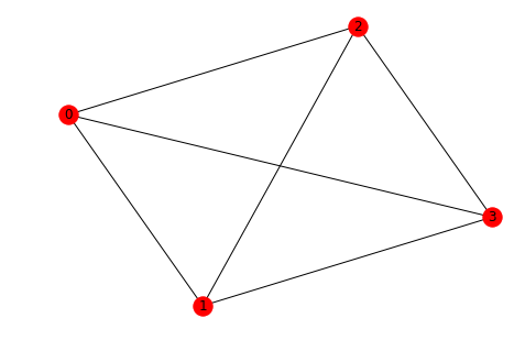
qubits = ideal_qc.qubits()
print('The qubits we will run on are', qubits)
graph = ideal_qc.qubit_topology()
nx.draw(graph, with_labels=True)
The qubits we will run on are [0, 1, 2, 3]
/anaconda3/lib/python3.7/site-packages/networkx/drawing/nx_pylab.py:611: MatplotlibDeprecationWarning: isinstance(..., numbers.Number)
  if cb.is_numlike(alpha):
Measure the quantum volume
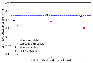
Here we will replicate Figure 2. of [QVOL0].
Start with the noiseless QVM
Caution, this is SLOW–it takes about 4 minutes.
[4]:
from forest.benchmarking.quantum_volume import measure_quantum_volume
[5]:
ideal_outcomes = measure_quantum_volume(ideal_qc, num_circuits=200, show_progress_bar=show_progress_bar)
100%|██████████| 200/200 [00:43<00:00,  4.25it/s]
100%|██████████| 200/200 [01:19<00:00,  2.52it/s]
100%|██████████| 200/200 [03:42<00:00,  1.08s/it]
Now use a noisy QVM
This is SLOW–it takes about 5 minutes, even with half the number of shots from above.
[6]:
noisy_outcomes = measure_quantum_volume(noisy_qc, num_circuits=200, num_shots=500, show_progress_bar=show_progress_bar)
100%|██████████| 200/200 [00:46<00:00,  4.24it/s]
100%|██████████| 200/200 [01:15<00:00,  2.50it/s]
100%|██████████| 200/200 [03:21<00:00,  1.01it/s]
[7]:
depths = np.arange(2, 5)
ideal_probs = [ideal_outcomes[depth][0] if depth in ideal_outcomes.keys() else 0 for depth in depths]
noisy_probs = [noisy_outcomes[depth][0] if depth in noisy_outcomes.keys() else 0 for depth in depths]

plt.axhline(.5 + np.log(2)/2, color='b', ls='--', label='ideal asymptote')
plt.axhline(2/3, color='black', ls=':', label='achievable threshold')
plt.scatter(np.array(depths) - .1, ideal_probs, color='b', label='ideal simulation')
plt.scatter(depths, noisy_probs, color='r', label='noisy simulation')
plt.ylabel("est. heavy output probability h_d")
plt.xlabel("width/depth of model circuit m=d")
plt.ylim(.4,1.0)
plt.xlim(1.8, 4.2)
plt.xticks(depths)
plt.legend(loc='lower left')
plt.show()
Use a QVM with different topologies
As explained in the references [QVOL0, QVOL1, QVOL2] the quantum volume is topology (or qubit connectivity) dependent. Here we show how to explore that dependence on the QVM.
[8]:
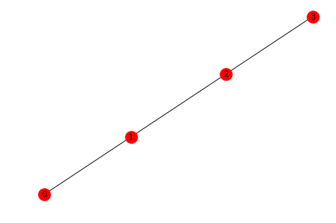
n = 4
path_graph = nx.path_graph(n)
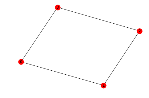
loop_graph = nx.cycle_graph(n)
four_pointed_star = nx.star_graph(n)
[9]:
nx.draw(path_graph, with_labels=True)
/anaconda3/lib/python3.7/site-packages/networkx/drawing/nx_pylab.py:611: MatplotlibDeprecationWarning: isinstance(..., numbers.Number)
  if cb.is_numlike(alpha):
[10]:
nx.draw(loop_graph, with_labels=True)
[11]:
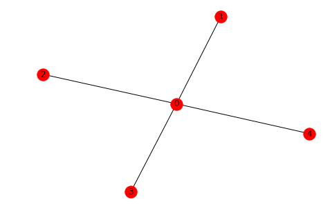
nx.draw(four_pointed_star, with_labels=True)
[12]:
from pyquil.api._quantum_computer import _get_qvm_with_topology
path_qc = _get_qvm_with_topology(name='path', topology=path_graph, noisy=True)
[13]:
path_outcomes = measure_quantum_volume(path_qc, num_circuits=200, num_shots=500, show_progress_bar=show_progress_bar)
100%|██████████| 200/200 [00:42<00:00,  4.81it/s]
100%|██████████| 200/200 [01:21<00:00,  2.81it/s]
100%|██████████| 200/200 [03:53<00:00,  1.18s/it]
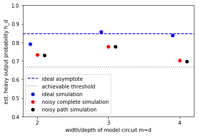
Compare to noisy complete topology
[14]:
depths = np.arange(2, 5)
ideal_probs = [ideal_outcomes[depth][0] if depth in ideal_outcomes.keys() else 0 for depth in depths]
noisy_probs = [noisy_outcomes[depth][0] if depth in noisy_outcomes.keys() else 0 for depth in depths]
path_probs = [path_outcomes[depth][0] if depth in path_outcomes.keys() else 0 for depth in depths]

plt.axhline(.5 + np.log(2)/2, color='b', ls='--', label='ideal asymptote')
plt.axhline(2/3, color='grey', ls=':', label='achievable threshold')
plt.scatter(np.asarray(depths) - .1, ideal_probs, color='b', label='ideal simulation')
plt.scatter(depths, noisy_probs, color='r', label='noisy complete simulation')
plt.scatter(np.asarray(depths) + .1, path_probs, color='black', label='noisy path simulation')
plt.ylabel("est. heavy output probability h_d")
plt.xlabel("width/depth of model circuit m=d")
plt.ylim(.4,1.0)
plt.xlim(1.8, 4.2)
plt.xticks(depths)
plt.legend(loc='lower left')
plt.show()
Run intermediate steps yourself
[15]:
from forest.benchmarking.quantum_volume import generate_abstract_qv_circuit, _naive_program_generator, collect_heavy_outputs
from pyquil.numpy_simulator import NumpyWavefunctionSimulator
from pyquil.gates import RESET
import time

def generate_circuits(depths):
    for d in depths:
        yield generate_abstract_qv_circuit(d)

def convert_ckts_to_programs(qc, circuits, qubits=None):
    for idx, ckt in enumerate(circuits):
        if qubits is None:
            d_qubits = qc.qubits()  # by default the program can act on any qubit in the computer
        else:
            d_qubits = qubits[idx]

        yield _naive_program_generator(qc, d_qubits, *ckt)


def acquire_quantum_volume_data(qc, programs, num_shots = 1000, use_active_reset = False):
    for program in programs:
        start = time.time()

        if use_active_reset:
            reset_measure_program = Program(RESET())
            program = reset_measure_program + program

        # run the program num_shots many times
        program.wrap_in_numshots_loop(num_shots)
        executable = qc.compiler.native_quil_to_executable(program)

        results = qc.run(executable)

        runtime = time.time() - start
        yield results


def acquire_heavy_hitters(abstract_circuits):
    for ckt in abstract_circuits:
        perms, gates = ckt
        depth = len(perms)
        wfn_sim = NumpyWavefunctionSimulator(depth)

        start = time.time()
        heavy_outputs = collect_heavy_outputs(wfn_sim, perms, gates)
        runtime = time.time() - start

        yield heavy_outputs
Generate (len(unique_depths) x n_circuits) many “Abstract Ckt”s that describe each model circuit for each depth.
[16]:
n_circuits = 100
unique_depths = [2,3]
depths = [d for d in unique_depths for _ in range(n_circuits)]
ckts = list(generate_circuits(depths))
print(ckts[0])
([array([0, 1]), array([0, 1])], array([[[[-0.55144177-0.26647286j,  0.25608208-0.41848682j,
           0.55437382+0.11126989j, -0.24805162+0.05435086j],
         [ 0.41850421-0.03852132j, -0.53379603-0.51061081j,
           0.26404218+0.40033292j,  0.15801984-0.15084347j],
         [-0.40802791+0.31687703j,  0.01503824+0.24504135j,
           0.17852483+0.25917974j,  0.57633624-0.49155065j],
         [-0.37207091-0.20721954j, -0.28645198-0.26702623j,
          -0.59009825-0.05516123j, -0.24902407-0.5019899j ]]],


       [[[ 0.0721541 +0.2574555j ,  0.44139907+0.09559298j,
           0.32209343+0.1954255j , -0.75505192-0.11180601j],
         [-0.04215926+0.38005476j, -0.80331064+0.15558321j,
           0.12962856+0.19247929j, -0.25682973+0.25387694j],
         [ 0.41663853+0.49404772j, -0.10656293-0.23819313j,
           0.2316722 -0.47365229j,  0.16001332-0.45892787j],
         [-0.52792383+0.29311608j,  0.09861876+0.22067494j,
          -0.34666698-0.63719413j, -0.19454456+0.11364139j]]]]))
Use the _naive_program_generator to synthesize native pyquil programs that implement each ckt natively on the qc.
[17]:
progs = list(convert_ckts_to_programs(noisy_qc, ckts))
print(progs[0])
DEFGATE LYR0_RAND0:
    -0.5514417662847406-0.26647286492053557i, 0.2560820842110857-0.41848681651537906i, 0.5543738175381981+0.1112698861629722i, -0.24805162392092533+0.054350859591478944i
    0.4185042068735709-0.03852132265800101i, -0.5337960273567897-0.5106108058052399i, 0.2640421819713798+0.4003329203692477i, 0.15801984183607665-0.15084346620705238i
    -0.408027909392624+0.31687703157097785i, 0.015038238995869325+0.24504135402018049i, 0.17852483272191516+0.2591797410324012i, 0.576336243741776-0.49155064672617377i
    -0.3720709110190956-0.20721953667663526i, -0.2864519762799716-0.2670262312865932i, -0.5900982511275752-0.0551612348120724i, -0.2490240699384845-0.5019899029508219i

DEFGATE LYR1_RAND0:
    0.07215410056104908+0.2574554986668327i, 0.4413990745932045+0.09559298457773703i, 0.3220934299476927+0.1954255019946097i, -0.7550519199163047-0.11180601062380173i
    -0.042159261292436585+0.3800547644756522i, -0.8033106407885078+0.1555832106222027i, 0.12962856172382972+0.1924792878027942i, -0.25682973276907545+0.2538769382460382i
    0.4166385333961749+0.4940477239306871i, -0.10656292914861569-0.23819313401134873i, 0.23167220332396365-0.4736522889207964i, 0.16001331852989328-0.4589278693974383i
    -0.5279238273136544+0.29311607971581133i, 0.09861875864941838+0.2206749435250735i, -0.3466669757393113-0.6371941326204252i, -0.19454456276883078+0.11364138547262737i

DECLARE ro BIT[2]
RZ(2.0898316269517103) 0
RX(pi/2) 0
RZ(0.2148303072673171) 0
RX(-pi/2) 0
RZ(-0.23883646690441696) 1
RX(pi/2) 1
RZ(1.8782549380583435) 1
RX(-pi/2) 1
CZ 1 0
RZ(1.2447911525773303) 0
RX(pi/2) 0
RZ(2.285972486228134) 0
RX(-pi/2) 0
RZ(-0.35540275892105777) 1
RX(-pi/2) 1
CZ 1 0
RX(pi/2) 0
RZ(-1.6322712380600009) 0
RX(-pi/2) 0
RZ(1.3075866603938913) 1
RX(pi/2) 1
CZ 1 0
RZ(1.3229164049932685) 1
RX(pi/2) 1
RZ(1.6990043194770588) 1
RX(-pi/2) 1
RZ(-0.16226001867169515) 1
MEASURE 1 ro[1]
RZ(-1.9258675572360893) 0
RX(pi/2) 0
RZ(1.7031448860980343) 0
RX(-pi/2) 0
RZ(1.2850615639649021) 0
MEASURE 0 ro[0]
HALT
Run the programs. This can be slow.
[18]:
num_shots=10
results = list(acquire_quantum_volume_data(noisy_qc, progs, num_shots=num_shots))
Classically simulate the circuits to get heavy hitters, and record how many hh were sampled for each program run.
[19]:
ckt_hhs = acquire_heavy_hitters(ckts)
Count the number of heavy hitters that were sampled on the qc
[20]:
from forest.benchmarking.quantum_volume import count_heavy_hitters_sampled
num_hh_sampled = count_heavy_hitters_sampled(results, ckt_hhs)
Get estimates of the probability of sampling hh at each depth, and the lower bound on that estimate
[21]:
from forest.benchmarking.quantum_volume import get_prob_sample_heavy_by_depth

results = get_prob_sample_heavy_by_depth(depths, num_hh_sampled, [num_shots for _ in depths])
results
[21]:
{2: (0.721, 0.6312984949959032), 3: (0.774, 0.6903521667943515)}
Use the results to get a lower bound on the quantum volume
[22]:
from forest.benchmarking.quantum_volume import extract_quantum_volume_from_results
qv = extract_quantum_volume_from_results(results)
qv
[22]:
2
[ ]: